In this second post, I will perform a membership analysis, that is, decide which stars in a region belong to a cluster based on Gaia data.

Membership analysis

Introduction

In this post, we will see how to decide which stars downloaded from a region actually belong to a cluster and which are field stars.

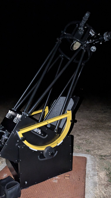
Last weekend, I took my 254 mm aperture Dobsonian telescope to the Trevinca Astronomical Centre to take advantage of the new moon. The Trevinca area has possibly the best skies in Galicia and north-western Spain, and it is always worth visiting to enjoy the starry sky. The sky wasn’t the best: smoke from nearby fires and a few clouds were a nuisance, but I was still able to enjoy quite a few objects. One object that always amazes me with binoculars or a telescope is the open cluster M37 (NGC 2009) in the constellation Auriga. The view through the telescope is breathtaking; a ‘wow’ is almost inevitable. I enjoyed it for several minutes, scanning the field little by little, with different magnifications, and more than a hundred stars can be identified in the field. Now I intend to learn more than what I saw through the eyepiece. Using data from Gaia DR3, I am going to download the stars in that field and decide which ones are really from the cluster and which ones are background stars in the same field. In the second instalment, I hope to be able to do some more analysis and learn how to interpret the results astrophysically.

M37 is the richest cluster in the constellation Auriga, with two other very interesting members, M36 and M38. According to some sources, it is known as the ‘Pebble Cluster’. According to some studies, it is approximately 4,500 light-years away. The light I saw this weekend appeared more or less when the Dolmen of Dombate was rising, the cathedral of megalithism in north-western Spain and one of my favourite places.

Origin and formation of open clusters

It is necessary to briefly explain the origin of an open cluster. An open cluster is a group of stars that formed together from the same molecular cloud of gas and dust. They are also known as “galactic clusters” because they are found in the plane of spiral galaxies, such as our Milky Way, where star formation is most active. The stars in open clusters tend to be young (< 1 billion years old) and consist of a few dozen to a few thousand stars. They are irregular in shape, and their stars are gravitationally bound.

The formation process of an open cluster begins with a large molecular cloud of gas and dust. Within this nebula, gravity causes some areas to contract and collapse. As these regions compress, the pressure and temperature increase, triggering nuclear fusion reactions and the birth of new stars. The newly formed stars emit a large amount of radiation and stellar winds that push the remaining gas and dust outwards. This process dissipates the original nebula, leaving behind a group of young stars that are visible as an open cluster.

Since the stars in an open cluster are not as strongly bound by gravity as those in globular clusters, gravitational interaction with other stars, gas clouds, or the centre of the galaxy itself causes the cluster to disperse over time and its stars to scatter.

Membership analysis

Membership analysis seeks to separate which stars truly belong to the cluster from field stars that are only in the same line of sight by chance. Cluster stars are stars that were born together, move together, and are at the same distance. Field stars are at different distances and move randomly; they do not appear to be related to each other or to the rest of the stars in the cluster. With this in mind, we will use three parameters to perform the membership analysis:

• pmRA and pmDEC (*proper motions**): stars in the cluster have very similar proper motions because they were born from the same molecular cloud and maintain similar velocities; the cluster moves as a whole through the Galaxy.
• parallax: the stars in the cluster are at the same distance, so they have similar parallaxes.

To perform the analysis using clustering algorithms, we can choose from several options. One that I have used in the past in business data environments is K-means (https://www.datacamp.com/en/tutorial/k-means-clustering-python). Another one used in this type of analysis is DBSCAN. I am going to use the latter for several reasons: the main one would be that DBSCAN does not need to know a priori how many groups it has to make, but rather discovers this automatically. Given that the purpose of this post is to show a possible application of Gaia data to analyse open clusters, I will not go into much more detail comparing it with other methods or improving the implementation of this algorithm (something I hope to do later). A few years ago, in a project for a company, I tried PyCaret (https://pycaret.org/) to validate the result with different algorithms, fine-tune the parameters, and orchestrate the entire pipeline in just 14 lines of code. I hope to review it soon in this context.

Description of the process

Jupyter notebook is uploaded to the repository of the project.

Environment configuration

I will carry out the development using Python in the same virtual environment that I created in the first post. All you need to do is add the popular scikit-learn library.

conda activate cluster_env

pip install scikit-learn

Data retrieval

Basic data from SIMBAD

I am going to reuse part of the code I wrote in the first Jupyter notebook. First, I retrieve the basic data (coordinates, size, etc.) from SIMBAD. With this result, we now have the necessary data to query Gaia (coordinates and size). When I run the query in SIMBAD, I get:

• Name: M 37
• Type: OpC
• RA: 88.077300º
• Dec: 32.543400º
• PmRA: 1.924 (mas/yr)
• PmDec: -5.648 (mas/yr)
• galdim_majaxis: 19.299999237060547 (arcmin)
• galdim_minaxis: 19.299999237060547 (arcmin)
• Radius: 9.649999618530273 (arcmin)
• Parallax: 0.666 (mas)

I already have the coordinates and size. With that, we will run the query on Gaia’s DR3 database. Keep in mind that the maximum size I am using is what SIMBAD returns. Perhaps I should expand the search radius a little more so as not to leave out any stars in the cluster from the query. The apparent field I saw through the telescope eyepiece did seem to be greater than 20 arcminutes.

Querying Gaia’s DR3 database

Now we are going to connect to the Gaia database and run a query based on the parameters obtained. On this occasion, I am taking the opportunity to create a function that I hope to refine and reuse later on.

The query ADQL already includes several quality filters:

• parallax > 0: I retrieve only stars with valid parallax
• parallax/parallax_error > 5: I filter only results with low parallax error
• pmra_error IS NOT NULL and pmdec_error IS NOT NULL: stars with reported errors in their proper motions
• phot_g_mean_mag < 20: stars brighter than magnitude 20
• ruwe < 1.4: stars with Renormalised Unit Weight Error <1.4, which guarantees the elimination of binary stars, acceptable astrometry, etc.

I run a simple query, reusing the previous code. This query returns an astropy.table.Table object, which I transform into a Pandas Dataframe using the to_pandas() method.

The query returns 1.783 stars

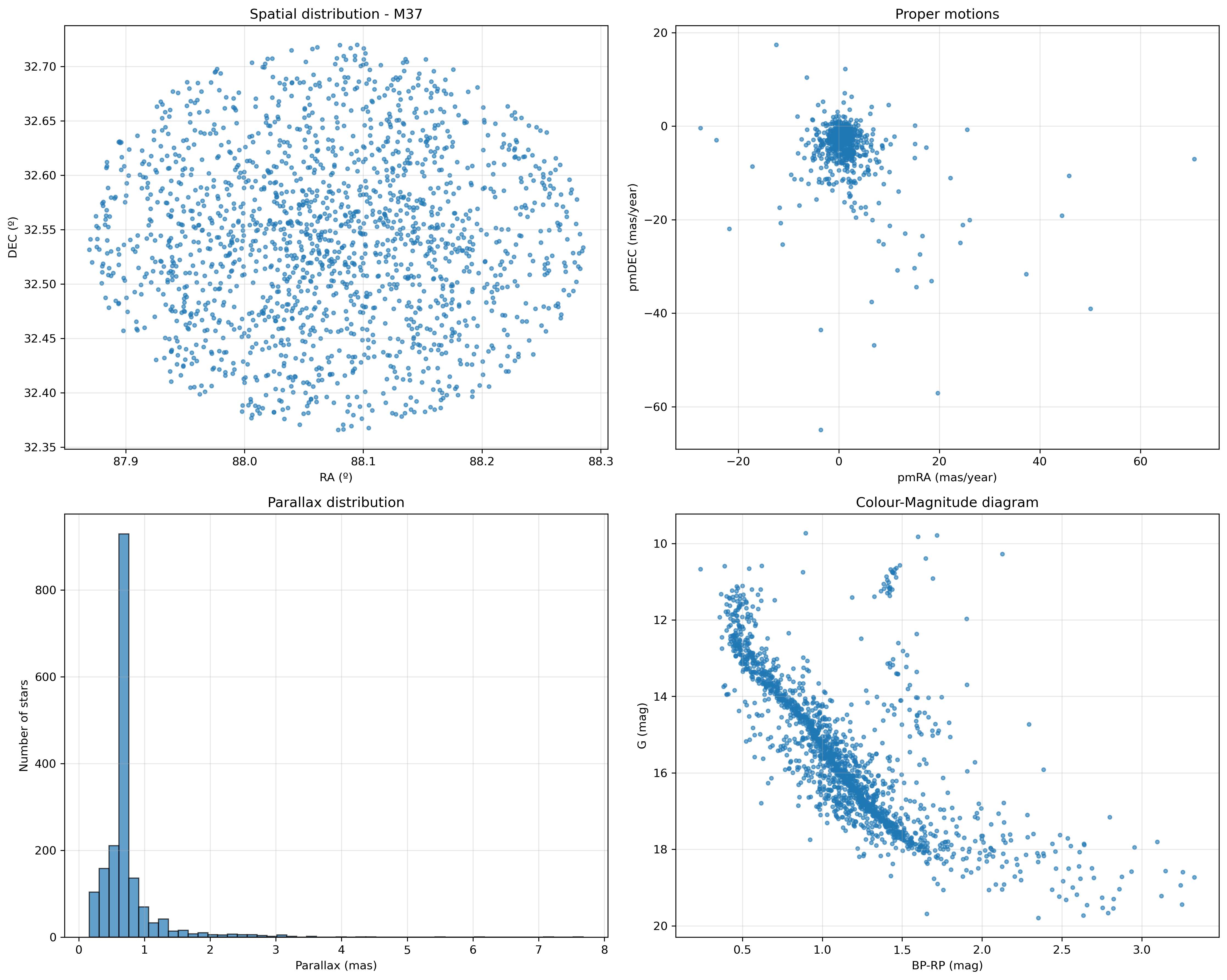
Some basic visualisations

Now I am creating some interesting graphs that will be useful in future analyses of the clusters. For the moment, they are only for illustrative purposes:

• celestial map
• diagram of proper motions
• histogram of parallaxes
• colour-magnitude diagram

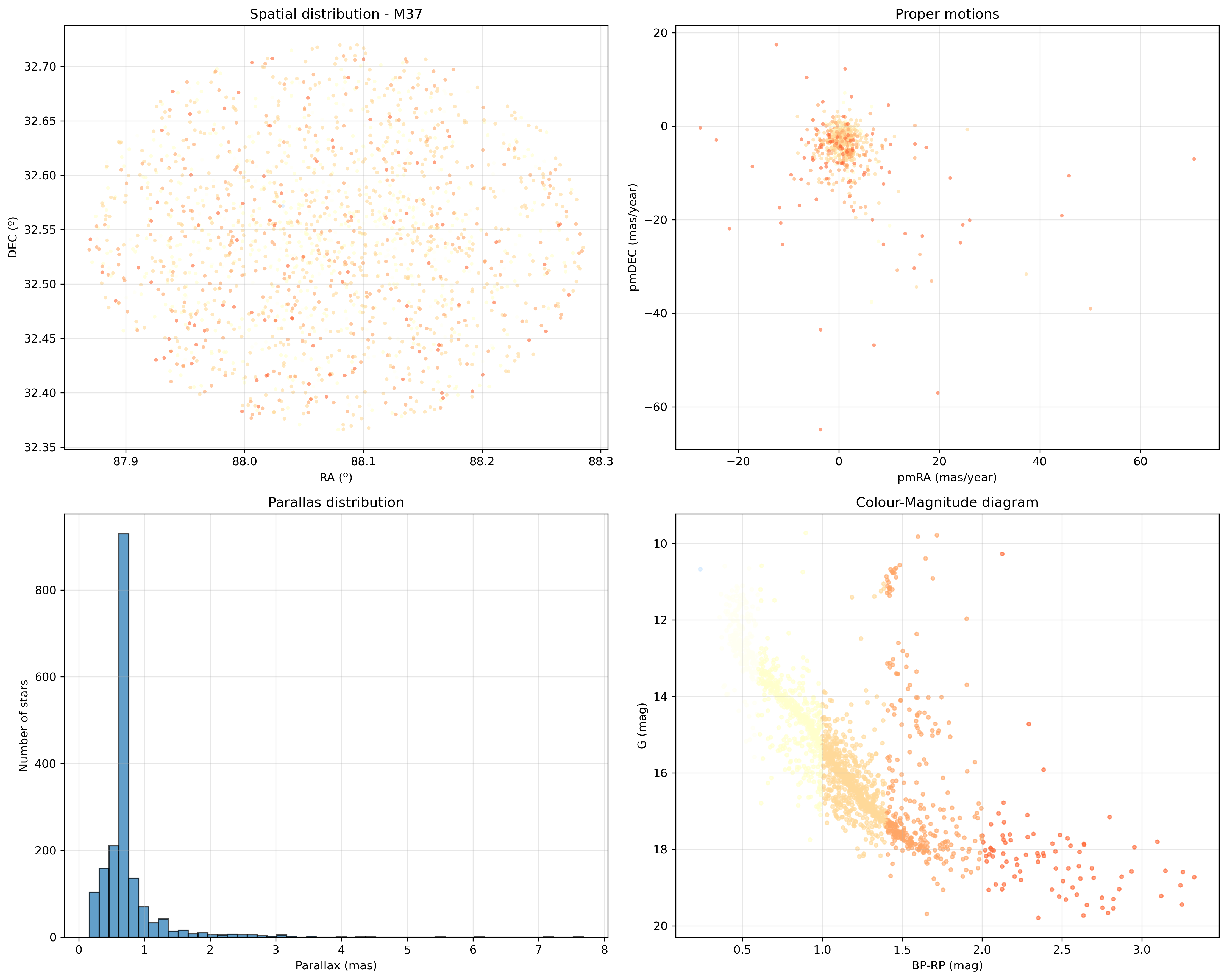
I also tried converting the BP and RP parameters to RGB colours so that I could paint the actual colour of each star in these graphs and see the result.

In future posts, I will delve deeper into the information that can be extracted from each one.

Membership analysis

Here comes the important part of today’s project: using clustering algorithms to determine which stars belong to the cluster. As I mentioned in the introduction, I will only test the DBSCAN algorithm for now.

I create a function to apply the algorithm. The parameters I am going to use are proper motions and parallax. As a first approximation, I believe these are the most important data and I will focus on them.

Following the usual steps in classification algorithm applications, I apply StandardScaler to scale the data and prevent one parameter from influencing more than another due to having higher absolute values. Then I apply the algorithm to the data. I used some parameters that I found in some reading, but they would require fine tuning to obtain the best results.

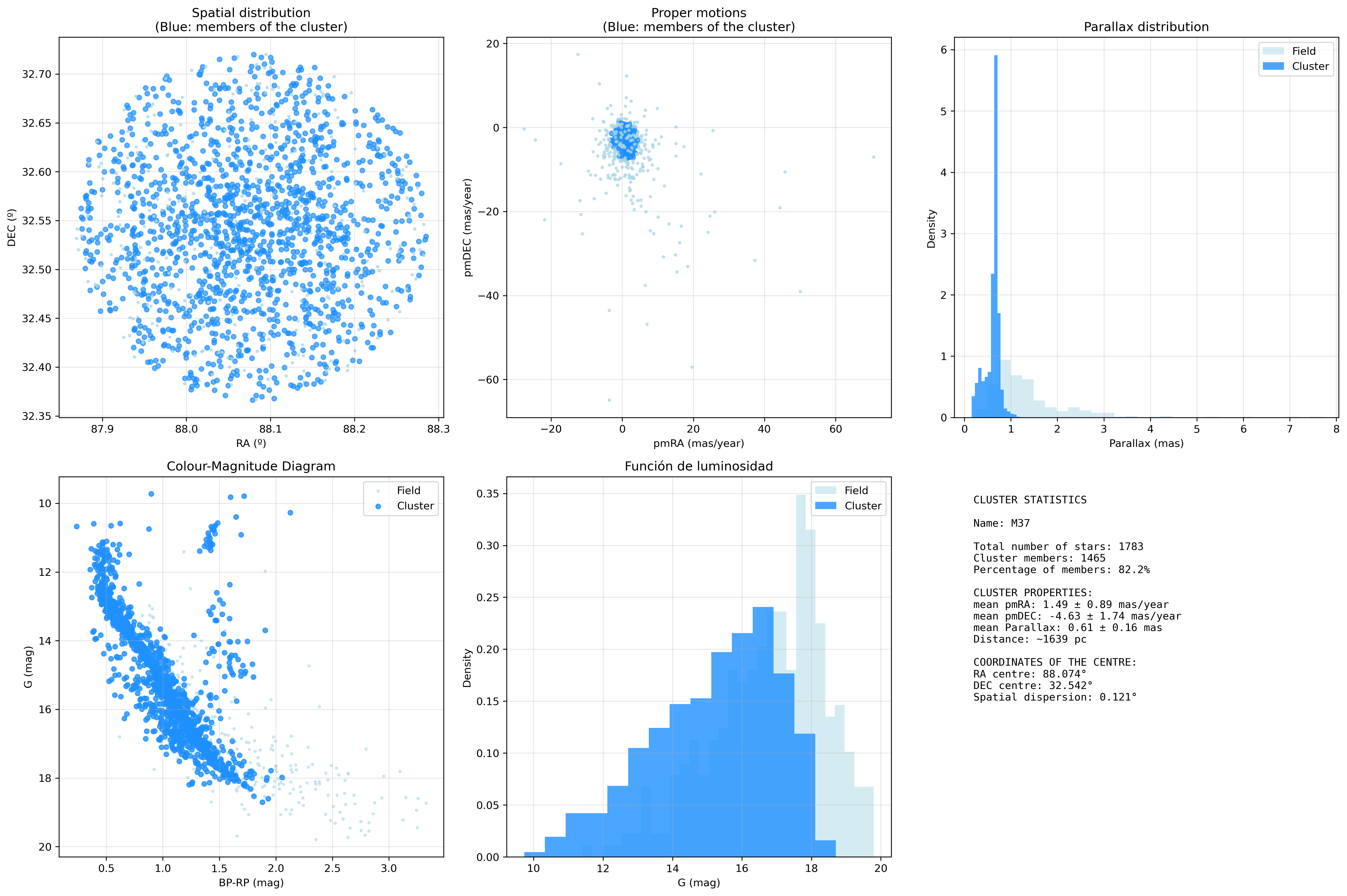
The final output of this block of code is a new column in the DataFrame indicating whether or not each of the downloaded stars is a member of the main cluster. This gives me 1,465 stars belonging to the cluster and 318 identified as noise.

In the next post, I will look for literature on other analyses of this cluster to compare and see if my approach seems correct.

Results

We now have a DataFrame with data on the stars belonging to the cluster with various parameters, from which we can draw some conclusions:

• RA of the centre: 88.074º
• DEC of the centre: 32.542º
• mean pmRA: 1.49 ± 0.89 mas/year
• mean pmDEC: -4.63 ± 1.74 mas/year
• mean Parallax: 0.61 ± 0.016
• mean distance: ~ 1,639 pc

Finally, we add the same visualisations as before, but marking which stars are members of the cluster.

Conclusions and next steps

This exercise is just another introduction to learning how to download and analyse data from an open cluster using the data available in Gaia DR3. These types of exercises help me in the process of discovering all the data available in the Gaia database, which attributes are most relevant in the study of open clusters, and how to process them. Also, although it will be described in part II of this article, discovering the scientific literature on this and other clusters, learning about the physical parameters that have been studied, and what are the open lines of research in this field.

With all this, I hope to make progress in acquiring a solid foundation for delving deeper into these fields and carrying out more complex analyses.

Regarding the analysis of M37, there are still quite a few points open that I hope to work on soon:

• Finding scientific literature with which to compare the results.
• Fine-tuning the parameters used in the algorithm.
• Comparing the results with other algorithms for membership analysis.

In the next post, I will attempt to conduct this research, compare the results obtained with other published studies, and advance the physical interpretation of the graphs and relevant information that can be obtained.